Location

2005/05/21 19:55:19 40.99N 14.51E 16 3.7 Italy

Arrival Times (from USGS)

Arrival time list

Felt Map

USGS Felt map for this earthquake

USGS Felt reports page for Intermountain Western US

Focal Mechanism

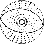
SLU Moment Tensor Solution 2005/05/21 19:55:19 40.99N 14.51E 16 3.7 Italy Best Fitting Double Couple Mo = 2.37e+21 dyne-cm Mw = 3.55 Z = 2 km Plane Strike Dip Rake NP1 100 50 -90 NP2 280 40 -90 Principal Axes: Axis Value Plunge Azimuth T 2.37e+21 5 190 N 0.00e+00 -0 280 P -2.37e+21 85 10 Moment Tensor: (dyne-cm) Component Value Mxx 2.26e+21 Mxy 3.99e+20 Mxz -4.06e+20 Myy 7.04e+19 Myz -7.15e+19 Mzz -2.34e+21 ############## ###################### ############################ ############################## #########-----------############## #####----------------------######### ###----------------------------####### ##--------------------------------###### ------------------- --------------#### #------------------- P ----------------### ##------------------ -----------------## ###--------------------------------------# #####------------------------------------# ######---------------------------------# #########----------------------------### ############---------------------##### ##################-------########### ################################## ############################## ############################ ###### ############# ## T ######### Harvard Convention Moment Tensor: R T F -2.34e+21 -4.06e+20 7.15e+19 -4.06e+20 2.26e+21 -3.99e+20 7.15e+19 -3.99e+20 7.04e+19 Details of the solution is found at http://www.eas.slu.edu/Earthquake_Center/NEW/20050521195519/index.html

INGV plot_3_st3.jpg INGV plot_6_st3_reviewed.jpg

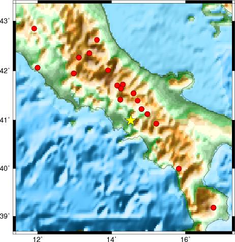
The focal mechanism was determined using broadband seismic waveforms. The location of the event and the station distribution are given in Figure 1.

Figure 1. Location of broadband stations used to obtain focal mechanism

Preferred Solution

      STK = 100
      DIP = 50
     RAKE = -90
       MW = 3.55
       HS = 2

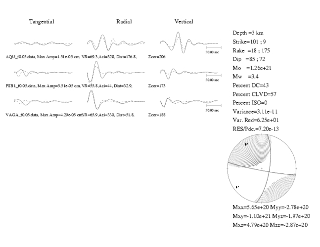
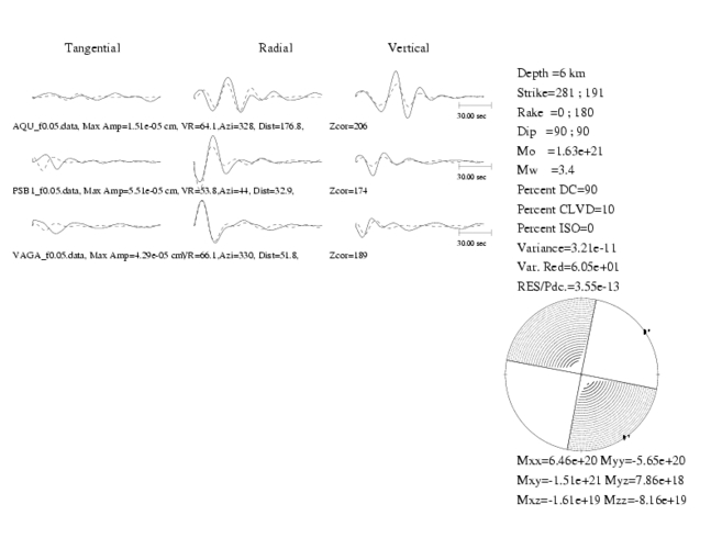
The solution given here is from waveform inversion of regional vaeforms from the INGV digital seismic stations.

Waveform Inversion

The program wvfgrd96 was used with good traces observed at short distance to determine the focal mechanism, depth and seismic moment. This technique requires a high quality signal and well determined velocity model for the Green functions. To the extent that these are the quality data, this type of mechanism should be preferred over the radiation pattern technique which requires the separate step of defining the pressure and tension quadrants and the correct strike.

The observed and predicted traces are filtered using the following gsac commands:

hp c 0.02 3
lp c 0.05 3

           DEPTH  STK   DIP  RAKE   MW    FIT
WVFGRD96    0.5   270    55   -90   3.48 0.3045
WVFGRD96    1.0   270    50   -90   3.49 0.2888
WVFGRD96    2.0   100    50   -90   3.55 0.3062
WVFGRD96    3.0   285    25   -75   3.63 0.2732
WVFGRD96    4.0   280    20   -80   3.67 0.2862
WVFGRD96    5.0   275    20   -85   3.68 0.2962
WVFGRD96    6.0    95    70   -85   3.68 0.2959
WVFGRD96    7.0    95    70   -85   3.68 0.2902
WVFGRD96    8.0    95    70   -85   3.70 0.2839
WVFGRD96    9.0    95    70   -85   3.69 0.2711
WVFGRD96   10.0   105    75   -75   3.67 0.2585
WVFGRD96   11.0   110    80   -70   3.66 0.2486
WVFGRD96   12.0   300    90    65   3.65 0.2438
WVFGRD96   13.0   310    80    60   3.66 0.2430
WVFGRD96   14.0   315    75    60   3.66 0.2431
WVFGRD96   15.0   315    75    60   3.66 0.2431
WVFGRD96   16.0   320    70    60   3.66 0.2432
WVFGRD96   17.0   325    65    65   3.67 0.2429
WVFGRD96   18.0   325    65    60   3.67 0.2422
WVFGRD96   19.0   320    65    60   3.67 0.1358
WVFGRD96   20.0   320    65    60   3.66 0.1351
WVFGRD96   21.0   320    65    65   3.72 0.2324
WVFGRD96   22.0   325    60    65   3.73 0.2318
WVFGRD96   23.0   325    60    65   3.73 0.2309
WVFGRD96   24.0   335    55    70   3.73 0.2300
WVFGRD96   25.0   330    55    70   3.74 0.2291
WVFGRD96   26.0   330    55    70   3.74 0.2282
WVFGRD96   27.0   330    55    70   3.74 0.2278
WVFGRD96   28.0   340    50    75   3.75 0.2273
WVFGRD96   29.0   335    50    75   3.76 0.2280
WVFGRD96   30.0   335    50    75   3.76 0.2287

The best solution is

WVFGRD96    2.0   100    50   -90   3.55 0.3062

The mechanism correspond to the best fit is

Figure 1. Waveform inversion focal mechanism

The best fit as a function of depth is given in the following figure:

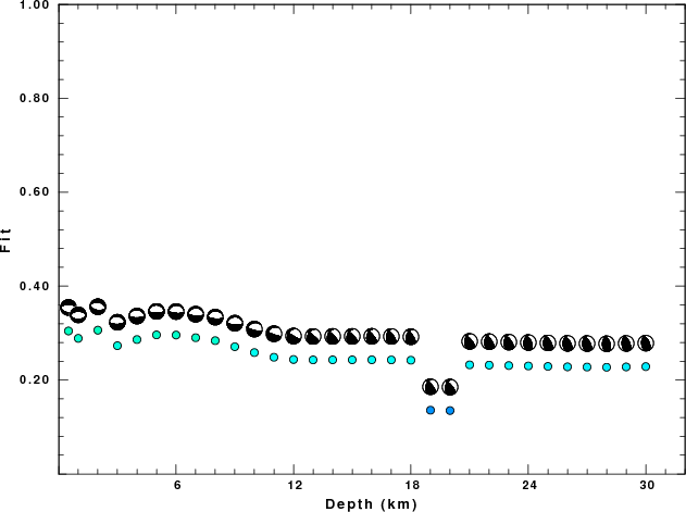
Figure 2. Depth sensitivity for waveform mechanism

The comparison of the observed and predicted waveforms is given in the next figure. The red traces are the observed and the blue are the predicted. Each observed-predicted componnet is plotted to the same scale and peak amplitudes are indicated by the numbers to the left of each trace. The number in black at the rightr of each predicted traces it the time shift required for maximum correlation between the observed and predicted traces. This time shift is required because the synthetics are not computed at exactly the same distance as the observed and because the velocity model used in the predictions may not be perfect. A positive time shift indicates that the prediction is too fast and should be delayed to match the observed trace (shift to the right in this figure). A negative value indicates that the prediction is too slow. The bandpass filter used in the processing and for the display was

hp c 0.02 3
lp c 0.05 3

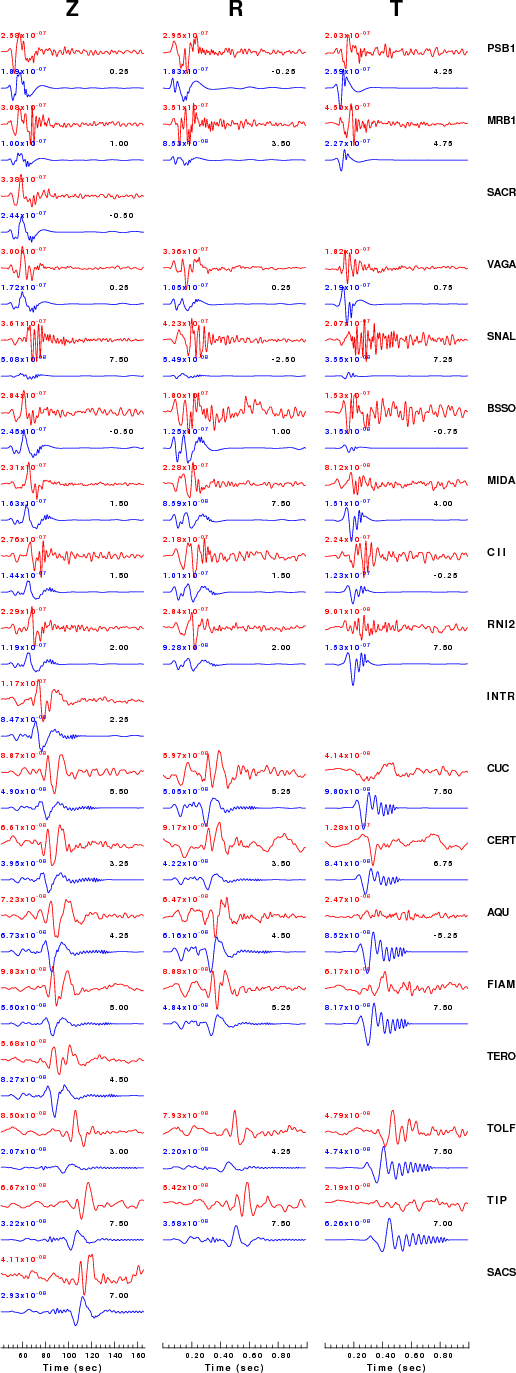
Figure 3. Waveform comparison for depth of 8 km

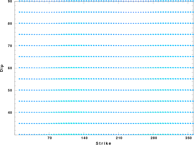
Focal mechanism sensitivity at the preferred depth. The red color indicates a very good fit to thewavefroms. Each solution is plotted as a vector at a given value of strike and dip with the angle of the vector representing the rake angle, measured, with respect to the upward vertical (N) in the figure.

First motion data

The P-wave first motion data for focal mechanism studies are as follow:

Sta Az(deg)    Dist(km)   First motion
PSB1       43   36 eP_+
MRB1       68   40 iP_C
SACR       19   48 eP_X
VAGA      333   53 iP_D
SNAL       97   58 iP_C
BSSO        6   62 iP_D
MIDA      343   76 eP_-
CII       348   83 eP_+
RNI2      339   85 eP_-
MRLC      107   86 eP_X
TRIV        2   86 eP_X
FRES        6  110 eP_X
INTR      336  125 eP_X
CUC       135  156 eP_+
CERT      310  167 iP_D
AQU       329  178 eP_X
FIAM      321  184 eP_D
TERO      338  197 iP_D
TOLF      300  242 eP_X
TIP       136  277 eP_X
CING      338  287 eP_+
SACS      315  299 eP_X
MURB      327  302 eP_X
CEL       158  325 eP_X
ARCI      310  327 eP_X

Quality control

The follwoing stations were not used because of excessive low frequency noise in the deconvolved waveforms: AMUR, GIUL, RNI2, SNAL, TRIV