Location

2004/12/05 01:52:38 48.20 8.10 0 5.2 Germany

Arrival Times (from USGS)

Felt Map

Focal Mechanism

USGS/SLU Moment Tensor Solution ENS 2004/12/05 01:52:38:0 48.20 8.10 0.0 5.2 Germany Stations used: CH.BNALP CH.BOURR CH.FUORN CH.SENIN CZ.DPC CZ.KHC CZ.NKC G.ECH GE.STU GE.WLF GR.BFO GR.BRG GR.BUG GR.CLL GR.CLZ GR.FUR GR.MOX GR.NOTT GR.UBBA IU.GRFO MN.TUE NL.HGN NL.WTSB OE.DAVA OE.KBA PL.KSP SL.CEY SL.CRES SL.LJU SX.NEUB SX.TANN Y4.LAU Y4.VAT Filtering commands used: cut a -30 a 180 rtr taper w 0.1 hp c 0.02 n 3 lp c 0.06 n 3 Best Fitting Double Couple Mo = 6.61e+22 dyne-cm Mw = 4.48 Z = 15 km Plane Strike Dip Rake NP1 20 85 -10 NP2 111 80 -175 Principal Axes: Axis Value Plunge Azimuth T 6.61e+22 3 66 N 0.00e+00 79 174 P -6.61e+22 11 335 Moment Tensor: (dyne-cm) Component Value Mxx -4.14e+22 Mxy 4.90e+22 Mxz -9.19e+21 Myy 4.34e+22 Myz 8.68e+21 Mzz -1.99e+21 ------------- -- P -------------#### ----- ------------######## ---------------------######### ----------------------############ -----------------------############ -----------------------############# T ##----------------------############# ####-------------------################# #########--------------################### ############-----------################### ################------#################### ########################################## ####################------############## ###################--------------####### #################--------------------- ###############--------------------- ##############-------------------- ###########------------------- #########------------------- #####----------------- -------------- Global CMT Convention Moment Tensor: R T P -1.99e+21 -9.19e+21 -8.68e+21 -9.19e+21 -4.14e+22 -4.90e+22 -8.68e+21 -4.90e+22 4.34e+22 Details of the solution is found at http://www.eas.slu.edu/eqc/eqc_mt/MECH.EU/20041205015238/index.html

Preferred Solution

The preferred solution from an analysis of the surface-wave spectral amplitude radiation pattern, waveform inversion and first motion observations is

      STK = 20
      DIP = 85
     RAKE = -10
       MW = 4.48
       HS = 15.0

The NDK file is 20041205015238.ndk The waveform inversion is preferred.

Moment Tensor Comparison

The following compares this source inversion to others

SLU OTHER

USGS/SLU Moment Tensor Solution ENS 2004/12/05 01:52:38:0 48.20 8.10 0.0 5.2 Germany Stations used: CH.BNALP CH.BOURR CH.FUORN CH.SENIN CZ.DPC CZ.KHC CZ.NKC G.ECH GE.STU GE.WLF GR.BFO GR.BRG GR.BUG GR.CLL GR.CLZ GR.FUR GR.MOX GR.NOTT GR.UBBA IU.GRFO MN.TUE NL.HGN NL.WTSB OE.DAVA OE.KBA PL.KSP SL.CEY SL.CRES SL.LJU SX.NEUB SX.TANN Y4.LAU Y4.VAT Filtering commands used: cut a -30 a 180 rtr taper w 0.1 hp c 0.02 n 3 lp c 0.06 n 3 Best Fitting Double Couple Mo = 6.61e+22 dyne-cm Mw = 4.48 Z = 15 km Plane Strike Dip Rake NP1 20 85 -10 NP2 111 80 -175 Principal Axes: Axis Value Plunge Azimuth T 6.61e+22 3 66 N 0.00e+00 79 174 P -6.61e+22 11 335 Moment Tensor: (dyne-cm) Component Value Mxx -4.14e+22 Mxy 4.90e+22 Mxz -9.19e+21 Myy 4.34e+22 Myz 8.68e+21 Mzz -1.99e+21 ------------- -- P -------------#### ----- ------------######## ---------------------######### ----------------------############ -----------------------############ -----------------------############# T ##----------------------############# ####-------------------################# #########--------------################### ############-----------################### ################------#################### ########################################## ####################------############## ###################--------------####### #################--------------------- ###############--------------------- ##############-------------------- ###########------------------- #########------------------- #####----------------- -------------- Global CMT Convention Moment Tensor: R T P -1.99e+21 -9.19e+21 -8.68e+21 -9.19e+21 -4.14e+22 -4.90e+22 -8.68e+21 -4.90e+22 4.34e+22 Details of the solution is found at http://www.eas.slu.edu/eqc/eqc_mt/MECH.EU/20041205015238/index.html

Cesca et al 2010 JGR Vol 115 B06304 do1:10.1029/JB006450 ENS 2004/12/05 01:52:38:0 48.11 8.07 11.7 5.1 Waldkirch, Germany Best Fitting Double Couple Mo = 7.08e+22 dyne-cm Mw = 4.50 Z = 11 km Plane Strike Dip Rake NP1 11 69 -27 NP2 111 65 -157 Principal Axes: Axis Value Plunge Azimuth T 7.08e+22 3 62 N 0.00e+00 56 156 P -7.08e+22 34 330 Moment Tensor: (dyne-cm) Component Value Mxx -2.13e+22 Mxy 5.06e+22 Mxz -2.67e+22 Myy 4.28e+22 Myz 1.91e+22 Mzz -2.15e+22 -----------### ----------------###### --------------------######## ------- -----------######### --------- P -----------########## ---------- -----------########## T -------------------------########## #-------------------------############## ##------------------------############## #####----------------------############### #######--------------------############### #########-----------------################ ############--------------################ ###############---------################ ###################-----################ ######################---###########-- #####################--------------- ###################--------------- ################-------------- ##############-------------- ##########------------ ####---------- Global CMT Convention Moment Tensor: R T P -2.15e+22 -2.67e+22 -1.91e+22 -2.67e+22 -2.13e+22 -5.06e+22 -1.91e+22 -5.06e+22 4.28e+22

Waveform Inversion

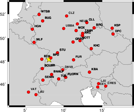
The focal mechanism was determined using broadband seismic waveforms. The location of the event and the and stations used for the waveform inversion are shown in the next figure.

Location of broadband stations used for waveform inversion

The program wvfgrd96 was used with good traces observed at short distance to determine the focal mechanism, depth and seismic moment. This technique requires a high quality signal and well determined velocity model for the Green functions. To the extent that these are the quality data, this type of mechanism should be preferred over the radiation pattern technique which requires the separate step of defining the pressure and tension quadrants and the correct strike.

The observed and predicted traces are filtered using the following gsac commands:

cut a -30 a 180
rtr
taper w 0.1
hp c 0.02 n 3 
lp c 0.06 n 3

The results of this grid search from 0.5 to 19 km depth are as follow:

           DEPTH  STK   DIP  RAKE   MW    FIT
WVFGRD96    1.0    20    85     5   4.09 0.4439
WVFGRD96    2.0    20    80    10   4.20 0.5576
WVFGRD96    3.0   200    85    10   4.24 0.6016
WVFGRD96    4.0   200    80    10   4.28 0.6264
WVFGRD96    5.0   200    80    10   4.31 0.6438
WVFGRD96    6.0   200    80    10   4.33 0.6589
WVFGRD96    7.0   200    80    10   4.36 0.6731
WVFGRD96    8.0    20    90   -20   4.39 0.6937
WVFGRD96    9.0    20    90   -20   4.41 0.7090
WVFGRD96   10.0   200    90    20   4.43 0.7225
WVFGRD96   11.0    20    85   -15   4.43 0.7379
WVFGRD96   12.0    20    85   -15   4.45 0.7507
WVFGRD96   13.0    20    85   -15   4.46 0.7587
WVFGRD96   14.0    20    85   -10   4.47 0.7644
WVFGRD96   15.0    20    85   -10   4.48 0.7665
WVFGRD96   16.0    20    85   -10   4.49 0.7650
WVFGRD96   17.0   200    90     5   4.51 0.7614
WVFGRD96   18.0    20    90     0   4.51 0.7588
WVFGRD96   19.0    20    90     0   4.52 0.7545
WVFGRD96   20.0   200    90    -5   4.53 0.7489
WVFGRD96   21.0    20    90     5   4.54 0.7431
WVFGRD96   22.0   200    90    -5   4.54 0.7353
WVFGRD96   23.0   200    90    -5   4.55 0.7268
WVFGRD96   24.0    20    90     5   4.56 0.7174
WVFGRD96   25.0   200    90    -5   4.57 0.7070
WVFGRD96   26.0    20    90     5   4.57 0.6970
WVFGRD96   27.0   200    90    -5   4.58 0.6872
WVFGRD96   28.0    20    90     5   4.59 0.6769
WVFGRD96   29.0    20    90     5   4.59 0.6664

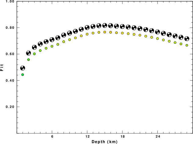
The best solution is

WVFGRD96   15.0    20    85   -10   4.48 0.7665

The mechanism correspond to the best fit is

Figure 1. Waveform inversion focal mechanism

The best fit as a function of depth is given in the following figure:

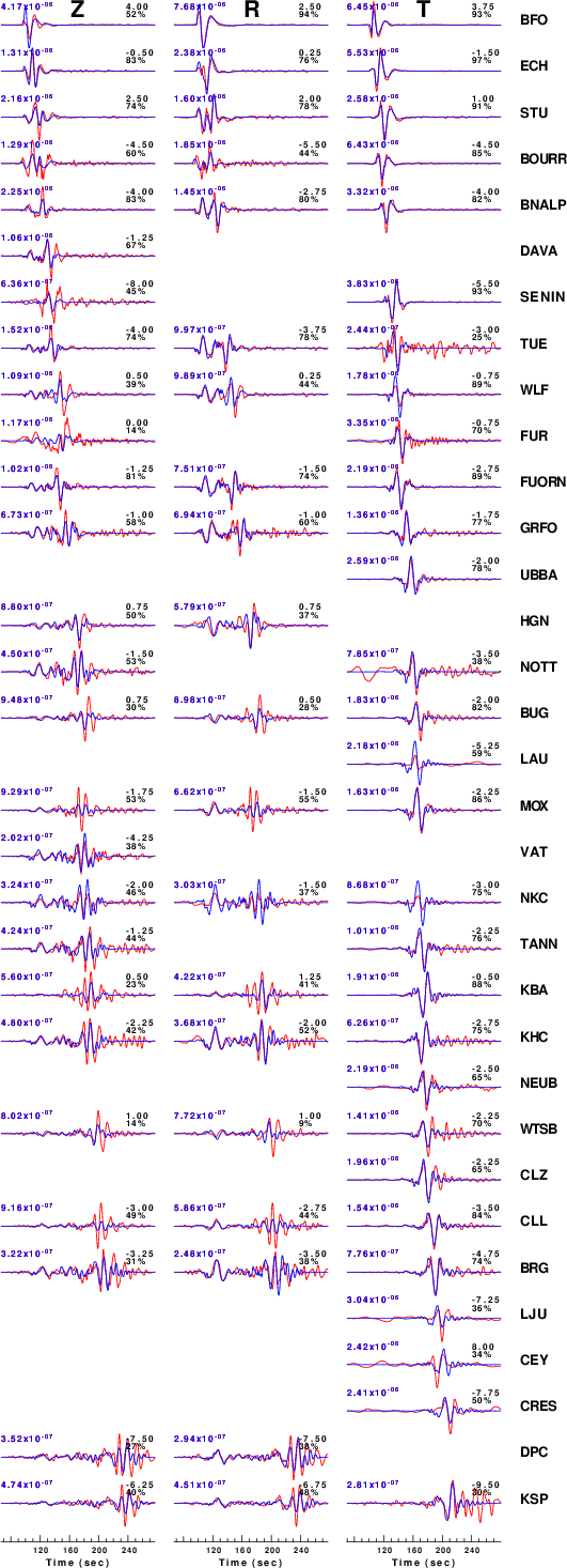
Figure 2. Depth sensitivity for waveform mechanism

The comparison of the observed and predicted waveforms is given in the next figure. The red traces are the observed and the blue are the predicted. Each observed-predicted component is plotted to the same scale and peak amplitudes are indicated by the numbers to the left of each trace. A pair of numbers is given in black at the right of each predicted traces. The upper number it the time shift required for maximum correlation between the observed and predicted traces. This time shift is required because the synthetics are not computed at exactly the same distance as the observed and because the velocity model used in the predictions may not be perfect. A positive time shift indicates that the prediction is too fast and should be delayed to match the observed trace (shift to the right in this figure). A negative value indicates that the prediction is too slow. The lower number gives the percentage of variance reduction to characterize the individual goodness of fit (100% indicates a perfect fit).

The bandpass filter used in the processing and for the display was

cut a -30 a 180
rtr
taper w 0.1
hp c 0.02 n 3 
lp c 0.06 n 3

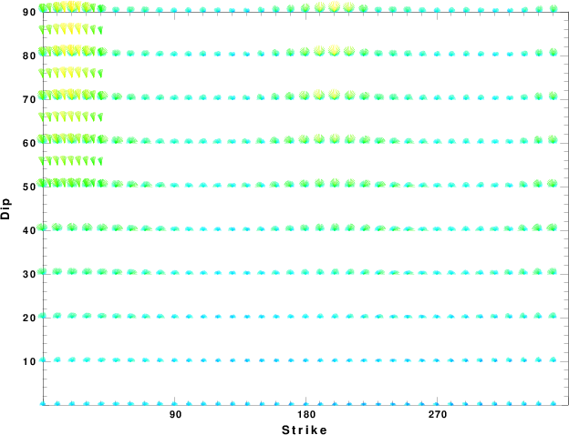
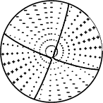
Figure 3. Waveform comparison for selected depth

Focal mechanism sensitivity at the preferred depth. The red color indicates a very good fit to thewavefroms. Each solution is plotted as a vector at a given value of strike and dip with the angle of the vector representing the rake angle, measured, with respect to the upward vertical (N) in the figure.

A check on the assumed source location is possible by looking at the time shifts between the observed and predicted traces. The time shifts for waveform matching arise for several reasons:

The origin time and epicentral distance are incorrect
The velocity model used for the inversion is incorrect
The velocity model used to define the P-arrival time is not the same as the velocity model used for the waveform inversion (assuming that the initial trace alignment is based on the P arrival time)

Assuming only a mislocation, the time shifts are fit to a functional form:

 Time_shift = A + B cos Azimuth + C Sin Azimuth

The time shifts for this inversion lead to the next figure:

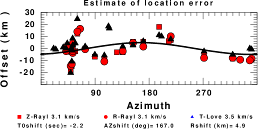
The derived shift in origin time and epicentral coordinates are given at the bottom of the figure.

Discussion

The Future

Should the national backbone of the USGS Advanced National Seismic System (ANSS) be implemented with an interstation separation of 300 km, it is very likely that an earthquake such as this would have been recorded at distances on the order of 100-200 km. This means that the closest station would have information on source depth and mechanism that was lacking here.

Acknowledgements

Dr. Harley Benz, USGS, provided the USGS USNSN digital data. The digital data used in this study were provided by Natural Resources Canada through their AUTODRM site http://www.seismo.nrcan.gc.ca/nwfa/autodrm/autodrm_req_e.php, and IRIS using their BUD interface.

Thanks also to the many seismic network operators whose dedication make this effort possible: University of Alaska, University of Washington, Oregon State University, University of Utah, Montana Bureas of Mines, UC Berkely, Caltech, UC San Diego, Saint L ouis University, Universityof Memphis, Lamont Doehrty Earth Observatory, Boston College, the Iris stations and the Transportable Array of EarthScope.

Velocity Model

The WUS used for the waveform synthetic seismograms and for the surface wave eigenfunctions and dispersion is as follows:

MODEL.01
Model after     8 iterations
ISOTROPIC
KGS
FLAT EARTH
1-D
CONSTANT VELOCITY
LINE08
LINE09
LINE10
LINE11
      H(KM)   VP(KM/S)   VS(KM/S) RHO(GM/CC)         QP         QS       ETAP       ETAS      FREFP      FREFS
     1.9000     3.4065     2.0089     2.2150  0.302E-02  0.679E-02   0.00       0.00       1.00       1.00    
     6.1000     5.5445     3.2953     2.6089  0.349E-02  0.784E-02   0.00       0.00       1.00       1.00    
    13.0000     6.2708     3.7396     2.7812  0.212E-02  0.476E-02   0.00       0.00       1.00       1.00    
    19.0000     6.4075     3.7680     2.8223  0.111E-02  0.249E-02   0.00       0.00       1.00       1.00    
     0.0000     7.9000     4.6200     3.2760  0.164E-10  0.370E-10   0.00       0.00       1.00       1.00

Quality Control

Here we tabulate the reasons for not using certain digital data sets

The following stations did not have a valid response files:

DATE=Thu Jul 3 03:25:20 CDT 2014

Last Changed 2004/12/05