Introduction

Creating the velocity model

The easiest way to create a velocity model is to modify an existing model. However for a simple model, you can use the CPS program mkmod96 to create the model.

However first create a place to work and then go that that directory:

mkdir EX1
cd EX1

Then do the following:

cps@cps-VirtualBox:~/EX1$ mkmod96
 Write creating model96 file for isotropic constant velocity layers, 1-D model
 Enter name of the earth model file
SCM.mod
  Model file is :SCM.mod
 Enter model comment
Simple crustal model
  Comment is    :Simple crustal model
 Enter 0 for flat earth model
       1 for spherical earth model
0
  Model flat/sph:           0
 Enter Velocity Model, EOF (CTRL D) to end:
  H     VP     VS      RHO    QP QS ETAP ETAS FREFP FREFS
 (km) (km/s) (km/s) (gm/cm^3) -- -- ---- ----  (Hz)  (Hz)
40 6 3.55 2.8 0 0 0 0 1 1
   40.0000000       6.00000000       3.54999995       2.79999995       0.00000000       0.00000000       0.00000000       0.00000000       1.00000000       1.00000000    
0 8 4.7 3.3 0 0 0 0 1 1
   0.00000000       8.00000000       4.69999981       3.29999995       0.00000000       0.00000000       0.00000000       0.00000000       1.00000000       1.00000000    
Ctrl_D
 Creating the model file:SCM.mod

Now let us look at the model

cat SCM.mod
MODEL.01
Simple crustal model
ISOTROPIC
KGS
FLAT EARTH
1-D
CONSTANT VELOCITY
LINE08
LINE09
LINE10
LINE11
      H(KM)   VP(KM/S)   VS(KM/S) RHO(GM/CC)     QP         QS       ETAP       ETAS      FREFP      FREFS    
    40.0000     6.0000     3.5500     2.8000   0.00       0.00       0.00       0.00       1.00       1.00    
     0.0000     8.0000     4.7000     3.3000   0.00       0.00       0.00       0.00       1.00       1.00

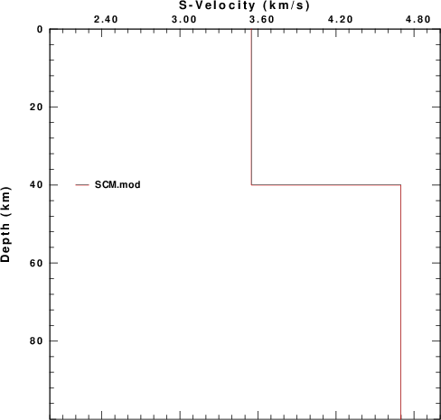
You will see that you have the correct model format.

Plotting the velocity model

To plot the model we can use the program shwmod96

shwmod96 -LEGIN -ZMAX 100 -K 2 SCM.mod

You can learn the meaning of the command line argiments by doing a

shwmod96 -h

In this case I want a legend inside the plot area, the maximum depth of the model is 100 km, the model is plotted using a red pen(2). The result is some output on the screen and also the CALPLOT file SHWMOD96.PLT. You can display this file ont he screen using the command

plotxvig < SHWMOD96.PLT

or you can make and Encapsulated PostScript file

plotnps -F7 -W10 -EPS -K < SHWMOD96.PLT > t.eps

and convert the EPS file to a PNG file for use with PowerPoint or a web page such as this

convert -trim t.eps -background white -alpha remove SCM.mod.png

Here the ImageMagick program convert converts the EPS to a PNG. The other part of the command removes transparency and forces the background to be white.

The result is the figure

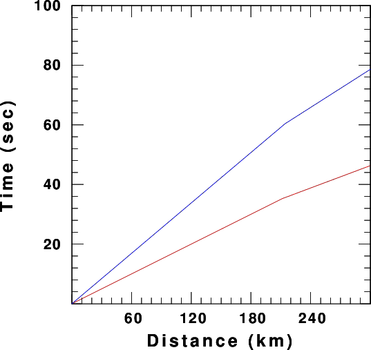
First arrival times using timmod96

Now that we have a model, run the program timmod96 as

timmod96 -P -K 2 SCM.mod                  Compute P-wave first arrivals and plot with pen 2 (red)
mv TIMMOD96.PLT P.PLT                     Rename the plot file
timmod96 -SV -K 4 SCM.mod                 Compute SV-first arrivals for surface source and receiver
                                           and plot using pen 4 (blue)
mv TIMMOD96.PLT S.PLT
cat P.PLT S.PLT > PS.PLT                  Concatenate the plot files (this is the way CALPLOT works
                                           unless the source code placed a new page command.
                                          This is how we make composite plots
plotnps -F7 -W10 -EPS -K < PS.PLT > t.eps
convert -trim t.eps -background white -alpha remove SCM.mod.PS.png   
                                          Convert to a PNG file

the result is the figure

The program timmod96 also creates a text file giving the first arrival times of P, SV and SH as a function of distance.
Just click on TIMMOD96.TXT to see the output.

Travel times for one ray

The program timmod96 was written to provide travel time tables for some location programs. Another useful program is time96 which give the first arrival time for one source and receiver. This is often used in a shell script to set theoretical P and S arrival times in Sac headers.

In this example the receiver is at the surface, the epicentral distance is 40 km, but the depth varies from 0 to 60 km and we want to compute the travel time (TIME) and the ray parameter (s/km) (RAYP) for these cases. Recall that for a flat laeyred medium, the ray parameter is just sin i/V where i is the angle of incidence and the V is the velocity where the angle is measured. The bash shell commands to do this are just

for DIST in 40
do
     for EVDP in 0 10 20 30 40 50 60
     do
          TIME=`time96 -DIST $DIST -EVDP $EVDP -T -P -M SCM.mod`
          RAYP=`time96 -DIST $DIST -EVDP $EVDP -RAYP -P -M SCM.mod`
          echo $DIST $EVDP $TIME $RAYP
     done
done

and the output is

40  0  e6.66666651 0.166666672
40 10  6.87184286 0.161690414
40 20  7.45355988 0.149071202
40 30  8.33333302 0.133333340
40 40  9.42809010 0.117851131
40 50 10.0902481  9.57615674E-02
40 60 10.9708700  8.20160136E-02

Exercise

Use timmod96 to plot P-wave first arrival times for source depths of 0, 20, 40, 60 and 80 km for the SCM model. Overlay the plots. Also plot the results using a reduction velocity of 6.0 km/s. The resulting plots should look like

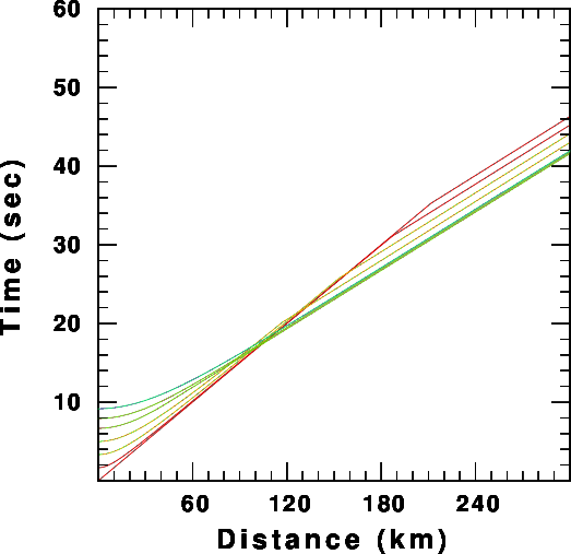
P-wave travel time as a function of source depth 0 to 80 km (colors red to blue). It is the change if shape with distance that permits location programs to determine source depth if station distances are such to sample the change in shape.

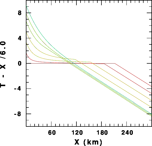
P-wave travel time as a function of source depth 0 to 80 km (colors red to blue) plotted with reduction velocity of 6.0 km/s.