
The propagator matrix technique as implemented in the Computer
Programs in Seismology sequence sprep96/sdisp96/sregn96
inherently assumes that the shear-wave velocity increases with
depth, although minor deviations are permitted. A characteristic
of such models is that the eigenfunction amplitudes that decay
exponentially with depth are largest near the surface of the
model.
There are other models for which this is not true. An extreme
case is that of a low velocity zone within a uniform wholespace,
or as presented here, a low velocity zone (LVZ) within a uniform
halfspace. For these extreme models one expects that
eigenfunctions should be contained withing the low velocity zone,
except for the halfspace case for which there will be something
like the classic Rayleigh wave propagating along the surface.
In isotropic media, surface waves arise by solving the
differential equations
for SH waves and

for P-SV waves with suitable boundary conditions. For normal use,
the boundary conditions are then the displacements (U) go to zero
as z goes to infinity and that the stresses at the surface be
zero. In such a case the solutions of the SH and P-SV problems are
called Love and Rayleigh waves, respectively.
The original surface wave codes of Computer Programs in
Seismology (CPS) that are in PROGRAMS.330/VOLIII/src, sprep96,
sdisp96, sregn96 and slegn96 for isotropic
media and tprep96, tdisp96, tregn96 and tlegn96
for transverse isotropic media, start computations from the bottom
halfspace up to the surface through the use of propagator matrices
for layers with constant parameters. One consequence of this is
that exponential eigenfunctions increase upward for the model.
This is not the appropriate behavior for the modes trapped within
the LVZ.
An alternative compurational procedure is to use reflection
rather than propagator matrices. Chen (1993) built upon the
technique of Kennett. Later Pei et al (2008) simplified the
procedure to use Generalized Reflection matrices. It was quickly
recognized the this technique could properly compute
eigenfunctions for a medium with a low velocity layer.
Several program in Computer Programs in Seismology use this
technique. For surface waves these are rregn96 and rlegn96
and for wavenumber integration there is rspec96 which can
handle a mixed stack of solid and fluid layers. At present rregn96
and rlegn96 only permit solid, isotropic layering.
The normal sequence of the surface wave dispersion codes is
indicated in this figure.

The rregn96 and rlegn96 replace the sregn96
and slegn96 in this flowchart. The other programs are not
changed. Just for completeness, the transverse isotropic problems
have the initial letter 't', e.g., tprep96, tdisp96,
tdpsrf96, tcomb96, tlegn96, tregn96,
tdpegn96, tdpder96 and tpulse96.
The procedure is to first compute the dispersion and then compute
the eigenfunctions. The program sdisp96 uses an extended
floating point implementation in software that avoids
overflow, and actually seems to get the correct
dispersion. So there is no corresponding rdisp96 program.
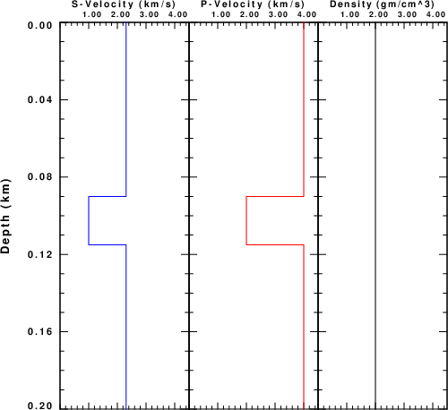
The model in Model96 format is
MODEL.01
LVZ Model with infinite Q, e.g., Q inverse = 0
ISOTROPIC
KGS
FLAT EARTH
1-D
CONSTANT VELOCITY
LINE08
LINE09
LINE10
LINE11
  H(KM) VP(KM/S) VS(KM/S) RHO(GM/CC)   QP   QS  ETAP  ETAS  FREFP  FREFS
  0.0900  4.0000  2.3090  2.0          0    0   0      0      1     1
  0.0125  2      1        2.0          0    0   0      0      1     1
  0.0125  2      1        2.0          0    0   0      0      1     1
  0.0100  4.0000  2.3090  2.0          0    0   0      0      1     1
 |
Using the velocity model, the following commands were executed to
get the dispersion:
#!/bin/sh

#prepare the data set
sprep96 -M SCMs.mod -R -DT 0.005 -NPTS 8191 -NMOD 10

# get the dispersion
sdisp96

# plot the dispersion but more importantly get the dispersion in ASCII form.
# The -K -1 forces a different color for each mode, with the fundamental
# in red and the highest in blue

sdpsrf96 -VMIN 0.0 -VMAX 2.5 -R -ASC -K -1


# convert the PLT file to a PNG using ImageMagick
DOPLTPNG  SDISPC.PLT
#!/bin/sh

for i
do
B=`basename $i .PLT`
plotnps -F7 -W10 -EPS -K < $i > t.eps
convert -trim t.eps -background white -alpha remove -alpha off ${B}.png
rm t.eps
done
The dispersion plot is
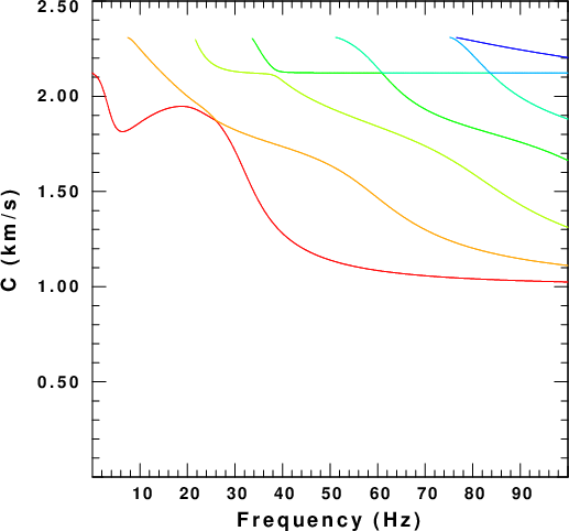 |
| Rayleigh wave phase velocities for the model
with a low velocity zone. The figure is color coded to
indicate the mode: Mode=0) (fundamental) is red, mode=6 is
blue. |
This is an interesting plot. Note the nearly horizontal phase velocity near 2.12295 km/s, which is the value expected for the classical halfspace Rayleigh wave for Vp=4.0 km/s and Vs=2.3098 km/s. The other phase velocity values are associated with modes trapped within the low velocity zone.
For the discussion of eigenfunctions that follows, we will focus
on the following dispersion values obtained from the call to
sdpsrf96.
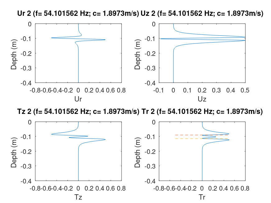
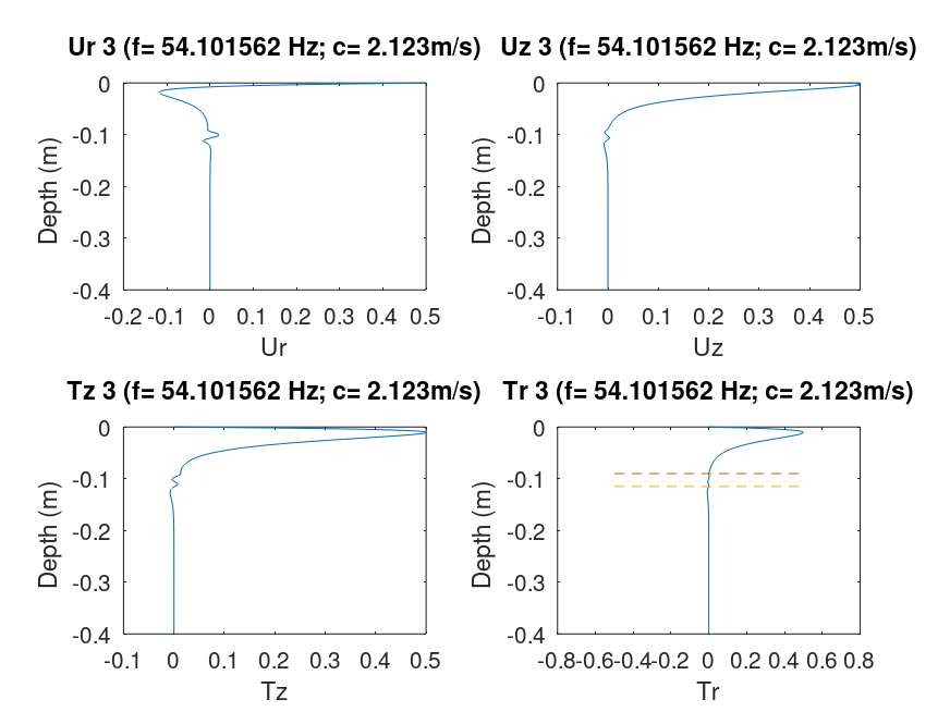
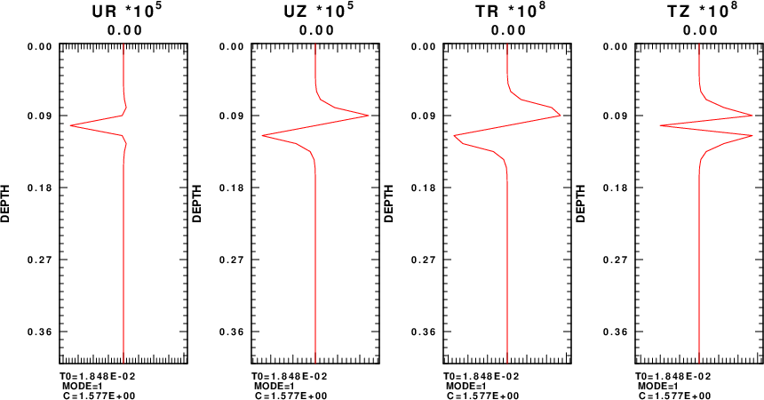
# RMODE NFREQ  PERIOD(S)          FREQUENCY(Hz)        C(KM/S)

#    0   236   0.1848375451E-01    54.10156250        1.112097914
#    1   236   0.1848375451E-01    54.10156250        1.577176773
#    2   236   0.1848375451E-01    54.10156250        1.897318721
#    3   236   0.1848375451E-01    54.10156250        2.122965625
#    4   236   0.1848375451E-01    54.10156250        2.279119456
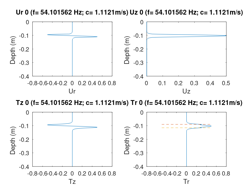
Eigenfunctions were computed using MATLAB code provided by Youhua Fan which was used for the paper
Liu, Xuefeng and Youhua Fan (2012). On the characteristics of high-frequency Rayleigh waves in stratified
half-space, Geophys. j. Int. 190, 1041-1057 doi: 10.1111/j.1365-246X.2012.05479.x
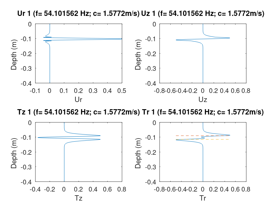
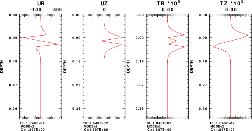
This code used generalized reflection matrices and an algorithm to define the correct eigenfunction. To determine the eigenfunctions for a given phase velocity and frequency, one selects a layer within which to compute the up- and down-going wave coefficients. The solutions for each are compared and one giving the smallest transformed stresses at the surface is selected as the appropriate eigenfunction. The normalized eigenfunctions are shown in the next figure. each frame displays the Ur,Uz, Tz and Tr eigenfunctions as a function of depth. The title line indicates the eigenfunction, mode, frequency and phase velocity. The horizontal dashed red lines in the Tr plots indicate the location of the low velocity zone.
 |
 |
 |
 |
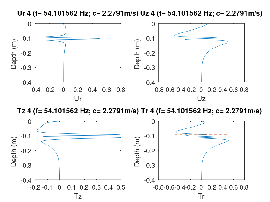 |
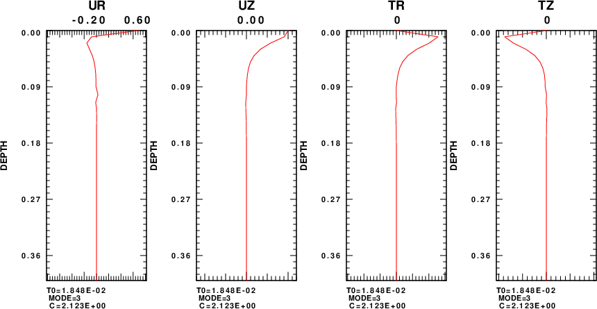
Focusing on the Uz eigenfunctions we see that the mode number corresponds to the number of zero crossings. We also see that for mode 3, for which the phase velocity was very close to the halfspace Rayleigh wave phase velocity that the eigenfunction amplitudes are largest near the surface, but that the correct number of zero crossing are there.
Starting with the discussion of Generalized Reflection matrices in Surface Waves in Layered Media (SWLM). I have created a FORTRAN code rregn96 for Rayleigh waves and rlegn96 for Love waves that computes eigenfunctions, group velocity, the energy integrals requires to get the AR and the phase velocity partials with respect to velocity and density. I have also created a Beigen_fc.m / Beigfuns.m following the Liu and Fan code, but using the definitions of SWLM as a test of the SWLM logic.
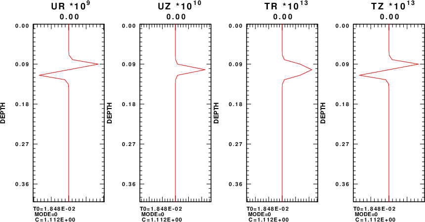
On February 5, 2024, I finally had a production run of regn96 to use to compare to the MATLAB results. In this program, the surface value of Uz is set to 1.0 and thus the eigenfunctions are not normalized. As recommended in the Fan code, one aspect of this implementation is that the code specifically uses the layer nearest the surface which has the lowest velocity. The eigenfunction plots for the five modes are given in the next figure. Each row shows the eigenfunciton plots for a given mode, which is indicated at the bottom of each plot.
 |
 |
 |
 |
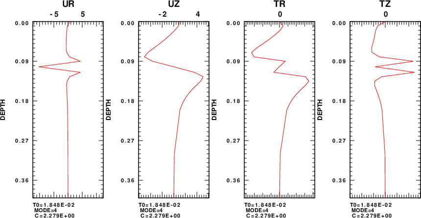 |
The eigenfunction shapes are the same as that from the MATLAB code. However we can now see the amplitudes.
It is useful to consider the contribution of each mode to a
synthetic. Recall that
 |
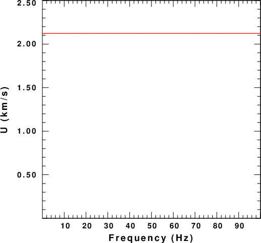
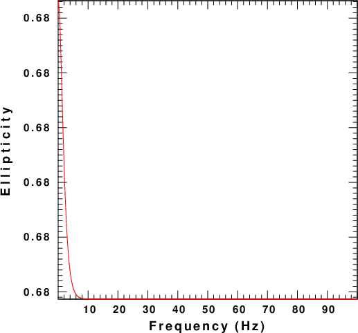
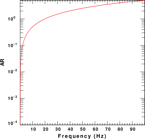
To evaluate the computations, the next set of figures displays
the phase velocity, C, group velocity,U, the surface
ellipticity, E, and the AR=A0 for all modes up to 100
Hz. The colors indicate the mode with the fundamental, mode=0, as
red, and the highest mode as blue.
|
 |
 |
 |
The next figure displays the dispersion for a uniform halfspace with the parameters of the top layer of the model given above.
 |
 |
 |
 |
| Original model |
Locked mode model |
MODEL.01 LVZ Model with infinite Q, e.g., Q inverse = 0 ISOTROPIC KGS FLAT EARTH 1-D CONSTANT VELOCITY LINE08 LINE09 LINE10 LINE11 H(KM) VP(KM/S) VS(KM/S) RHO(GM/CC) QP QS ETAP ETAS FREFP FREFS 0.0900 4.0000 2.3090 2.0 0 0 0 0 1 1 0.0250 2 1 2.0 0 0 0 0 1 1 0.0850 4.0000 2.3090 2.0 0 0 0 0 1 1 0.9000 4.0000 2.3590 2.0 0 0 0 0 1 1 |
MODEL.01 LVZ Model with infinite Q, e.g., Q inverse = 0 for locked mode ISOTROPIC KGS FLAT EARTH 1-D CONSTANT VELOCITY LINE08 LINE09 LINE10 LINE11 H(KM) VP(KM/S) VS(KM/S) RHO(GM/CC) QP QS ETAP ETAS FREFP FREFS 0.0900 4.0000 2.3090 2.0 0 0 0 0 1 1 0.0250 2 1 2.0 0 0 0 0 1 1 0.0850 4.0000 2.3090 2.0 0 0 0 0 1 1 0.9000 4.0000 2.3590 2.0 0 0 0 0 1 1 5 10 5 2 0 0 0 0 1 1 |
 |
 |
 |
 |
This distribution has two sub-directories: SECTION_001 for a
source depth of 0.001km and SECTION_100 for a source depth of
0.100km. The script DOIT in each directory computes the Greens
functions for point forces and for an isotropic moment tensor by
wavenumber integration. Thus all P and S waves are included to
represent a real data set. The script DOEGN computes the
theoretical phase velocities. The user then runs do_pom
to perform a phase velocity stack. Thus program creates the
CALPLOT file POM96.PLT and the shell script prototype POM96CMP
which uses the eigenfunctions computed by DOEGN. This script is
then hand edited to define the pen color and width.
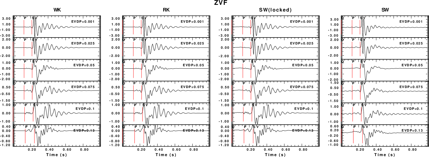
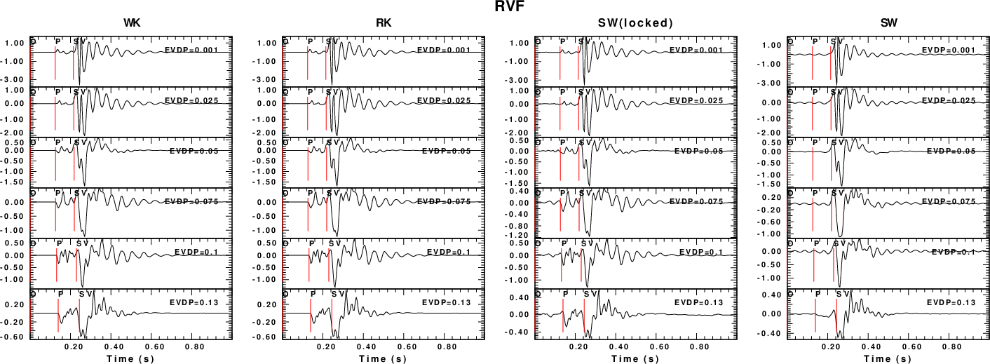
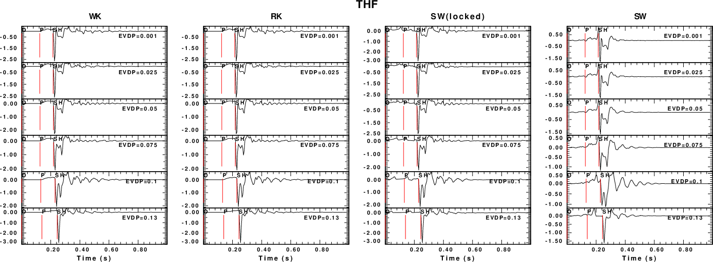
The ZVF and RHF record sections recorded at the surface are shown
in the next figure.
 |
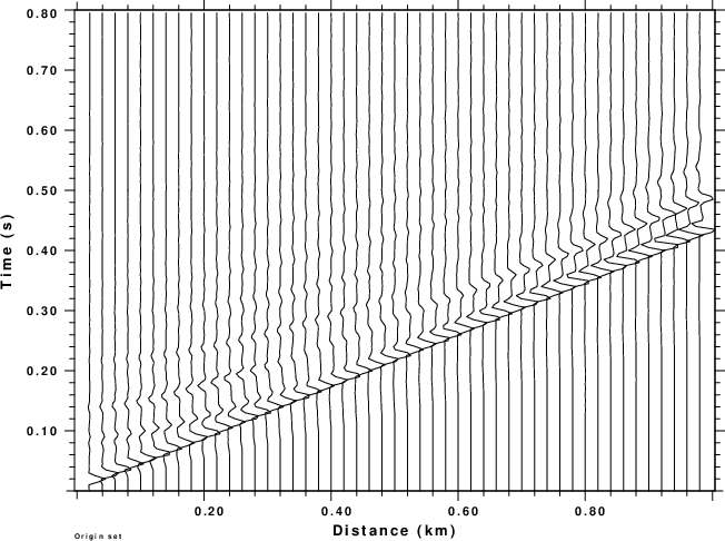 |
| ZVF record section | THF record section |
As expected the large arrival propagates with a velocity of about
2.2 km/s, which is close to the S-wave velocity outside of the
LVZ.
The next step is to perform a p-omega analysis using do_pom to
estimate the phase velocities. The sequence of operations is as
follows for vertical motions recorded at the surface due to a
point vertical force:
do_pom *.ZVF

[do_pom uses the following button sequence: Select all traces, MinPer of 0.01 sec, MaxPer of 2.0 sec, Nray 500, Vmin 0.010 km/sm Vmax 5.000 km/s, X-Axis Frequency Type Rayleigh and Length of 2.]

DOEGN
[Edit the POM96CMP so that the call to sdpegn96 to add 0=-K 0 -W 0.05 at the end to read
sdpegn96 -X0  2.00 -Y0  1.00 -XLEN  6.00 -YLEN  6.00 -XMIN  9.96 -XMAX 100. -YMIN  0.01 -YMAX 5.00 -FREQ -R -C -NOBOX -XLOG -YLIN -K 0 -W 0.05 ]

sh ./POM96CMP

cat POM96.PLT SREGNC.PLT > 001.PLT
../DOPLTPNG 001.PLT
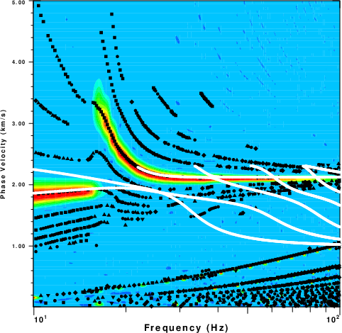
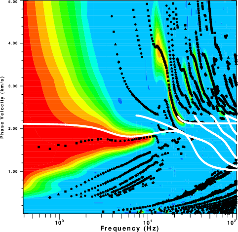
In this set of operations the theoretical dispersion is plotted
on top of the experimentally determined dispersion. The 100.png so
created is shown in this figure.
 |
 |
| Phase velocity analysis for the ZVF Green's
function |
Phase velocity analysis for the THF Green's
function |
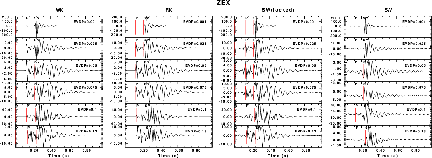
Here the ZEX Green's function is considered which is due to an
isotropic moment tensor source to represent signals generated by
an explosion at depth, which is the expected type of source in a
mine. The ZEX record section recorded at the surface is
shown in the next figure.
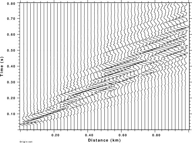 |
| ZEX record section |
The sequence of operations is as follows for vertical motions
recorded at the surface due to the isotropic moment tensor source
at depth:
do_pom *.ZEX

[do_pom uses the following button sequence: Select all traces, MinPer of 0.01 sec, MaxPer of 2.0 sec, Nray 500, Vmin 0.010 km/sm Vmax 5.000 km/s, X-Axis Frequency Type Rayleigh and Length of 2.]

DOEGN
[Edit the POM96CMP so that the call to sdpegn96 to add 0=-K 0 -W 0.05 at the end to read
sdpegn96 -X0  2.00 -Y0  1.00 -XLEN  6.00 -YLEN  6.00 -XMIN  9.96 -XMAX 100. -YMIN  0.01 -YMAX 5.00 -FREQ -R -C -NOBOX -XLOG -YLIN -K 0 -W 0.05 ]

sh ./POM96CMP

cat POM96.PLT SREGNC.PLT > 100.PLT
../DOPLTPNG 100.PLT
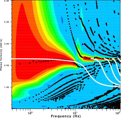
The 100.png so created is shown in this figure.
 |
| Phase velocity stack for ZEX Green's
functions at a source depth of 0.100 km. |
The purpose of the synthetic record sections was to determine
what might be observed in real data. For the shallow source, one
sees evidence of the LVZ at the lower frequencies, but at higher
frequencies the surface classic Rayleigh wave phase velocity is
seen in the vertical ZVF traces. For the SH in the THF traces,
there is a set of arrivals approaching the velocity of the S-wave
velocity of the cap. In both there are strong continuations of the
higher modes into the leaky modes.
The ZEX Green's functions for the deeper source are a bit more
interesting. This source will only generate P waves with phase
velocities greater than 2 km/s. Note that some of these will be
converted to S waves at the P-wave travels from the LVZ into the
higher velocity medium. However none will give rise to the low
velocity S waves in the LVZ. Thus the measured dispersion is hard
to model using surface wave theory.
As mentioned above, a thicker model with a high velocity base was
used for a locked mode approximation. In this case the leaky modes
of the simple case become ordinary modes that can be analyzed.
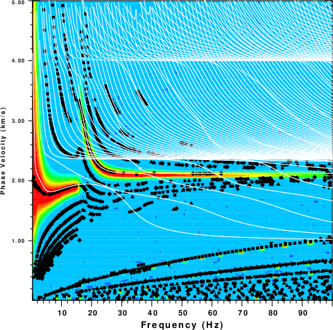
The locked mode method is still a modal superposition technique which means that it can only represent signals having phase velocities less than the S-velocity in the halfspace, which was 5 km/s. Thus one should be able to model some of the features shown in the phase velocity plots of the complete synthetics. In this set of plots a linear frequency axis is used rather than logarithmic.
One obvioous feature of these plots is that the number of modes is significantly greater. Note that there are apparent horizontal trends with velocities near 4.0 km/s and 2.4 km/s whose effect to to create the body wave arrivals.
In the ZVF figure for the 1m source depth, the feature seen above
at a frequency of about 20 Hz and phase velocity of 2.8km/s, which
was ascribed to a leaky mode is not modeled. In all cases
the very low frequency fundamental mode value is not well modeled.
If the record section had extended out to a greater
distance, then beter estimated would have resulted from the
procedure.
 |
 |
| Phase velocity analysis for the ZVF Green's
function |
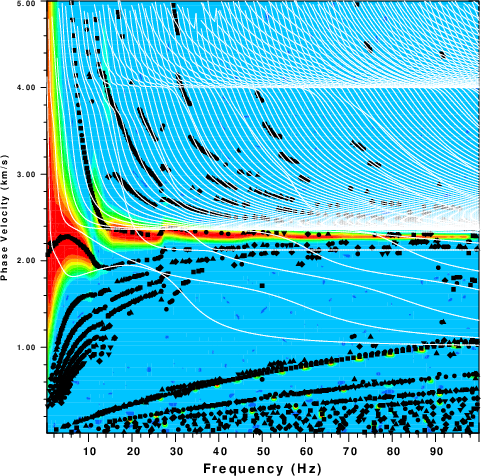
Phase velocity analysis for the THF Green's
function |
For the deeper source, we see that more of the features seen in
the phase velocity analysis of the ZEX traces correspond to modes.
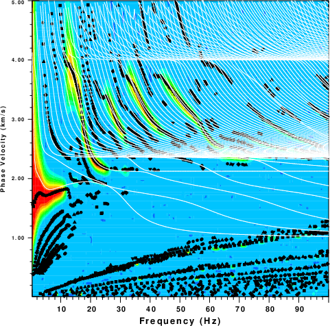 |
| Phase velocity stack for ZEX Green's
functions at a source depth of 0.100 km. |
The sregn96/slegn96 codes were developed 40 year ago and
are well tested. The challenge of properly handling a model with a
significant low velocity zone require some intuition of what the
various parameters should actually be. This the reason for the
extra step of computing synthetics by modal superposition. The
agreement with wavenumebr integration results was a necessary step
in validating the new rregn96/rlegn96 codes.
Since every tutorial needs a tarball of the run, the 075.tgz unpacks to
gunzip -c 075.tgz | tar tvf -
-rwxr-xr-x rbh/rbh         766 2024-02-20 13:50 LSW.075/DOIT
-rwxr-xr-x rbh/rbh         693 2024-02-20 10:52 RK.075/DOIT
-rwxr-xr-x rbh/rbh         722 2024-02-20 13:51 SW.075/DOIT
-rwxr-xr-x rbh/rbh         693 2024-02-20 10:54 WK.075/DOIT
DOIT script in each subdirectory will give the Green's functions for a source depth of 0.075 km in the LVZ model.