Introduction
The velocity model format used in Computer Programs in Seismology
has long had the provision for conveniently incorporating a layered
atmosphere from the viewpoint of having the source or receiver
depth of 0 km be at the air-solid interface. This is
accomplished by the use of negative layer thicknesses to indicate
layering above a reference datum, usually the surface of the earth.
The computational codes use a coordinate system with the z=0
corresponding to the top of the model, and positive z corresponds to
greater depth. With the convention of layers above the datum
used in the model formats, the synthetic seismogram codes does the
book keeping necessary to convert the user view to that required for
computation.
As an interesting exercise, we will consider the wavefields
generated in the air (pressure field) and in the solid (velocities)
from point explosion sources in the air and solid. In addition the
pressure field in the atmosphere is also computed for various
dislocation sources.
The positions of the sources (small red dots) and receivers (large
blue dots) are shown in Figure 1. Although in actuality
observations are made at the surface, the framework indicated here
could be used to drive detailed atmospheric models. To predict
pressure fields at large distances, ray theory may be the most
efficient technique for high frequency signals, since the
computational effort inherent in wave-number integration would be
too great. So the idea here is to prototype the expected
pressure signals on a hemisphere about the source, and then
eventually to use a representation theorem to uses these motions as
input to a ray theory or other numerical technique.
The receivers in Figure 1 are at a distance of 20 km from the
coordinate system origin (the intersection of the vertical and
horizontal axes). For position in the air, only the pressure field
will be measurable, while at the surface, pressure and ground
motions can be determined.
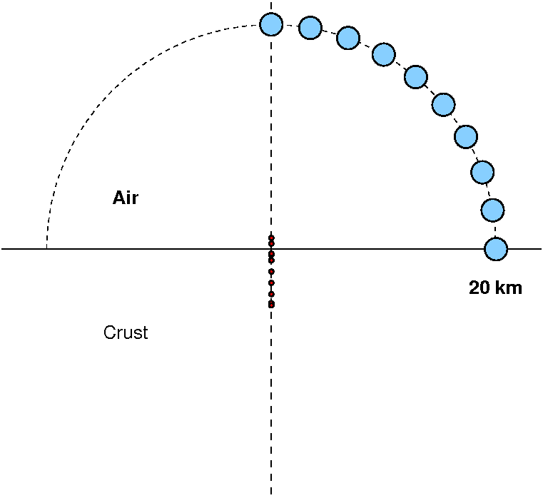 |
Fig. 1. Distribution of
receivers (blue) and sources. The receivers are at
radial distance of 20 km from origin. The sources are at
depths of -1, -0.5, 0, 0.5, 1, 2, 3, 4 and 5 km. The
negative source depth indicates a source in the air.
|
The velocity model used is very simple: a single layer
atmosphere overlying a solid half-space. The model96 file descript is given
in the file crust-atmos.mod:
MODEL.01
Simple Crust Atmosphere model
ISOTROPIC
KGS
FLAT EARTH
1-D
CONSTANT VELOCITY
LINE08
LINE09
LINE10
LINE11
  H(KM) VP(KM/S) VS(KM/S) RHO(GM/CC)   QP   QS  ETAP  ETAS  FREFP  FREFS
-40.0000  0.3000  0.0000  0.0012 0.00  0.00  0.00  0.00  1.00  1.00
 40.0000  6.0000  3.5000  2.8000 0.00  0.00  0.00  0.00  1.00  1.00
Here you can see the use of the negative depth to indicate that a
user specification of a source depth of 1 km means that the depth in
the internal model will be 41 km from the top, or 1 km into the
solid. Note that this model is just used for testing. The
density of air at sea level is about 0.00129 gm/cc.
Processing
The processing is performed with the script DOIT
and the graphics by the script DOFIG in
the sub-directory FIGURES.
The DOIT script treats the model as two halfspaces which means that
there will be no returns from the top and bottom inerfaces.
Discussion
Effect of source depth
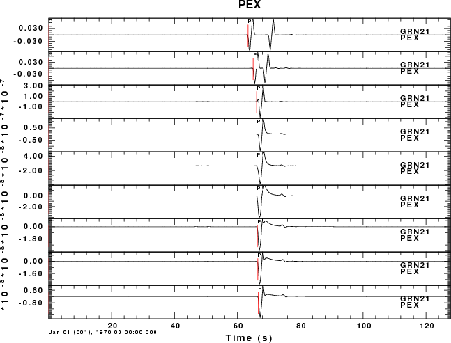
the first example considers the pressure field measured in the
atmosphere at an angle of 80 degrees measure from the horizontal.
The observation is at a distance of 3.473 km and an elevation of
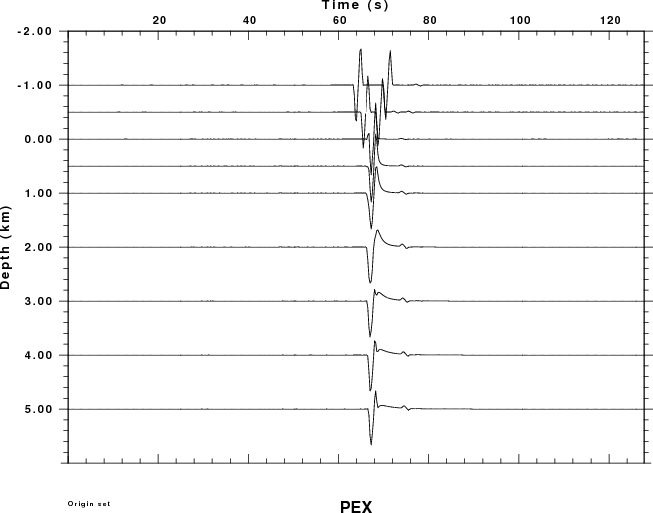
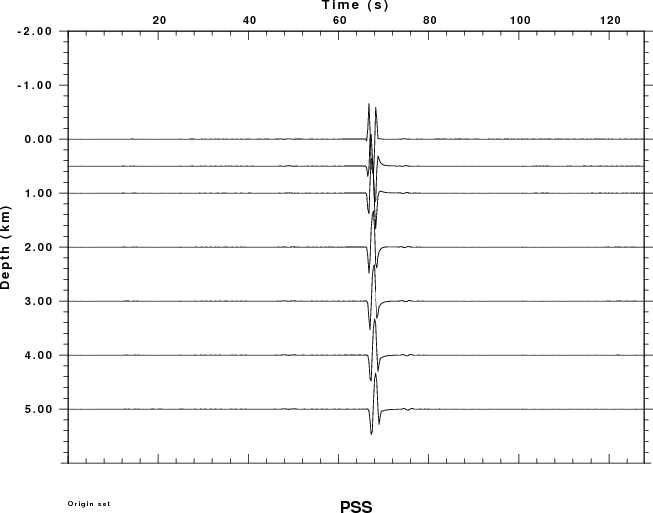
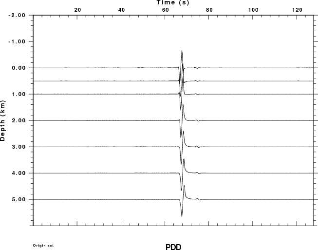
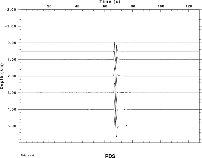
19.696 km. The plots shown below present the Greens functions
for a moment of 1.0E+20 dyne-cm. A relative amplitude scale is used.
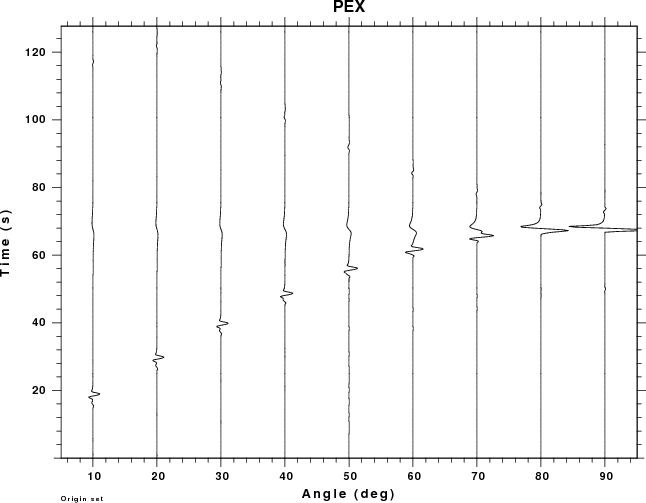
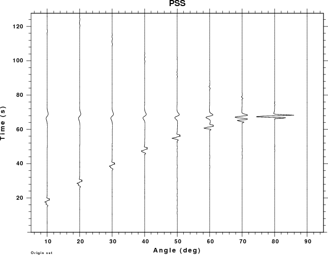
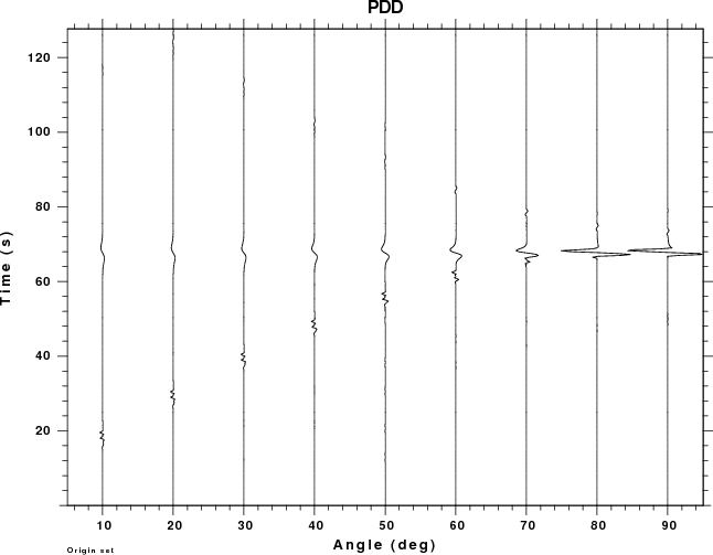
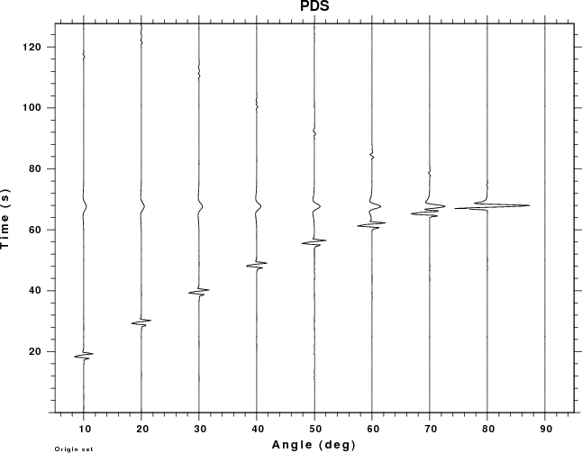
Since dislocation sources cannot occur in the atmosphere, the plots
for the PSS, PDD and PDS Greens functions have no data for negative
receiver depths (e.g., in the air).
Focus first on the PEX Green function. For atmospheric sources
the signal consists of two pulses, which are the direct signal and
the reflection from the solid surface.
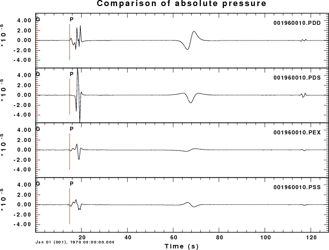
If a absolute amplitudes were plotted, the observations for the
buried sources would appear as straight lines because the
amplitudes are so small compared to the wavefield due to an
atmosphere source (for an explosion). For the PEX Greens
functions the largest negative amplitudes are -0.07, -0.07,
-2.9E-07, -1.38E-07, -7.73E-08, -4.01E-08, -3.53E-08, -2.99E-08
and -2.73E-07 for source depths of -1, -0.5, 0, 1, 2, 3, 4 and 5
km. This lower amplitudes for the buried source can be understood
from ray theory for which the spectral amplitude should vary as
Mo/[4 pi rhos alphas3
] [rhos alphas / rhoa
alphaa ]1/2 for an explosion source
in the solid observed in the atmosphere, and
Mo/[4 pi rhoa alphaa3
] for an explosion source in the atmosphere and observed in
the atmosphere. The ratio of the amplitudes is just
[ rhos alphas3
] / [ rhoa alphaa3
] [rhoa alphaa / rhos alphas
]1/2 which is factor of about 1.1E+6,
which is the difference in the amplitudes shown in the second
figure.
|
Absolute Pressure Plot
|
 |
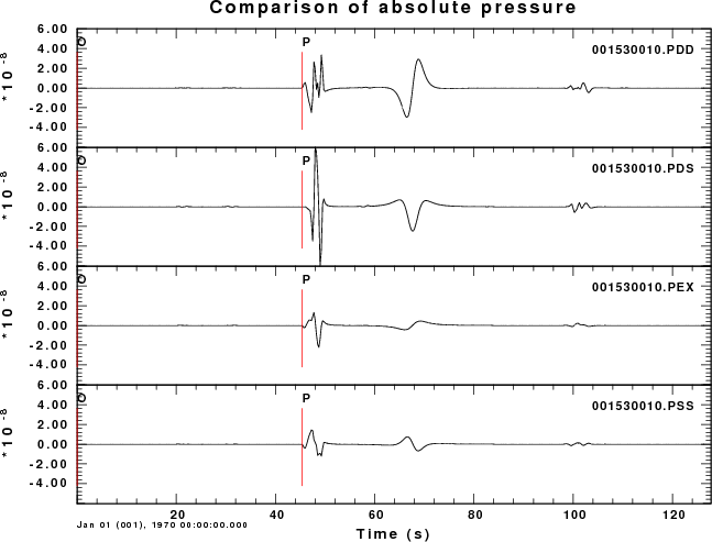
Radiated pressure field of a 1 km deep source
This example considers the pressure field at all sensors in the
atmosphere, whose location is defined by the angle with respect to
the horizontal. An angle of 90 degrees indicates a receiver directly
above the source. In the following set of plots, all traces use the
same scale so that amplitudes can be compared. the larges
amplitude are above the source.
For this set of examples we see two arrivals for small angles.
Focusing on the receiver closest to the surface, e.g., angle of 10
degrees, the first arrival at 14 sec travel time consists of the
P-wave propagating through the solid (about 3 seconds) which then
propagates 3.4 km in air (11 sec). The low frequency arrival at
about 68 sec is due to the air wave generated by the surface
deformation above the source.
Comparison of excitation from 1 km deep sources
|
10 degree angle
|
40 degree angle
|
 |
 |
Last changed March 24, 2012