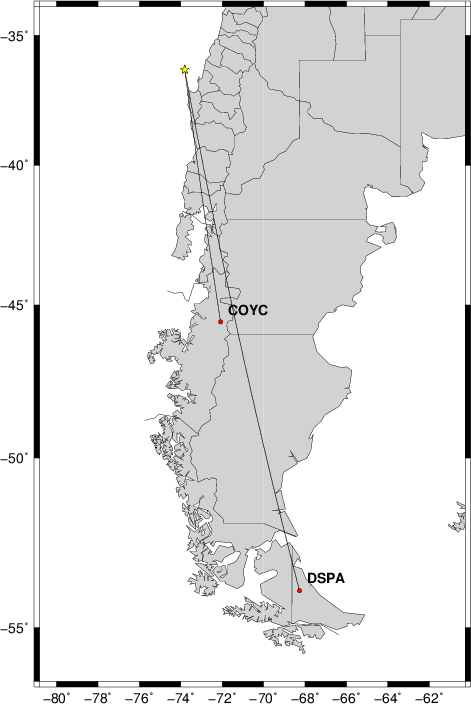
Fig 1. Location of earthquake (star) and the two stations to be used in the two station technique for getting phase velocity.
Fig 1. Location of earthquake (star) and the two stations to be used in the two station technique for getting phase velocity. |
The assumptions of a two-station technique are that
(a) a single surface mode is observed at both stations,
(b) that both stations be on the same great circle path which means that the contribution of the source phase to the observed phase is the same, and
that there be good signal-to-noise in the observed signal, which requires that the path from the source to the stations not be one of low amplitude.
The event selected is that of 2015/06/20 02:10 in Central Chile. The GCMT solution for this earthquake was
201506200210A NEAR COAST OF CENTRAL CH

  Date: 2015/ 6/20   Centroid Time:  2:10:13.4 GMT
  Lat= -36.35  Lon= -74.10
  Depth= 12.0   Half duration= 3.9
  Centroid time minus hypocenter time:  6.3
  Moment Tensor: Expo=25  2.940 0.058 -3.000 -1.190 -4.100 -0.713
  Mw = 6.4    mb = 0.0    Ms = 6.4   Scalar Moment = 5.25e+25
  Fault plane:  strike=9    dip=18   slip=84
  Fault plane:  strike=196    dip=72   slip=92
The azimuth from the source to each station was
2015.171.021121.G.COYC.BHZ (0):
           AZ             172.4544
2015.171.021317.AI.DSPA.BHZ (1):
           AZ             169.3566
To test whether there was sufficient amplitude at the source, I used the program sdprad96 and the CUS velocity model (this is just a sensitivity test and the model should not be too important) to create the theoretical radiation patterns at a period of 20 seconds. The result of executing the shell script DOIT.RADPAT is given in Figure 2.
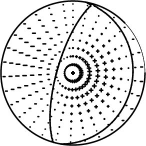 Fig. 2a. Predicted first motion plot for the GCMT mechanism |
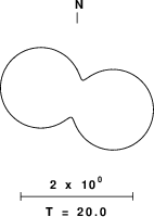 Fig. 2b. Predicted radiation pattern for the 20 second, fundamental mode Rayleigh wave |
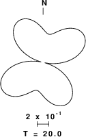 Fig. 2c. Predicted radiation pattern for the 20 second, fundamental mode Love wave |
This indicates that the path to the stations is not nodal, but that there might be lower amplitudes. Note that the Rayleigh wave pattern usually changes shape more with period than the Love wave pattern.
The reason for the interest in the radiation pattern was prompted by a plot of the instrument corrected ground motion in Figure 3.
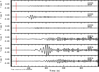 Fig. 3. Comparison of ground motions at COYC (distance of 1033 km) to those at DSPA (distance of 2001 km). The BHR, BHT and BHZ represent the radial, transverse and vertical motions. |
| DOITZ for the Rayleigh wave | DOITT for the Love wave |
#!/bin/bash

#####
#    apply a two station techique to get phase velocity for the
#    two stations on the same great circle path
#####
#    the steps are as follow
#    1. Measure the group velocity dispersion from the two traces
#       and then save the one which is better defined and which
#       has the greatest range of periods
#       do_mft -G *BHZ
#       a) pick the dispersion
#       b) click on the "Match"
#          The screen output will show how sacmat96 is called, e.g.,
#          /Users/rbh/PROGRAMS.310t/PROGRAMS.330/bin/sacmat96 -F 2015.171.021121.G.COYC.BHZ -D disp.d -AUTO
#          we will not use the match dispersion, jus the command line
#          We need to use the same command for both stations. We are really interested in the disp.d file

do_mft -G *BHZ
#####
#   when Match is selected in do_mft, a command line is printed on the terminal
#   showing the syntax for executing sacmat96. We apply the disp.d to
#   all traces of the same time so that all are processed with the
#   same range of periods
#####
for TRACE in *BHZ
do
	sacmat96 -F ${TRACE} -D disp.d -AUTO
done

#####
#    as a result of this the hase matched traces will have an 's' appended
#    to the file name
#####

#####
#    Before determining the phase velocities, we cut the waveforms from
#    the original length because this 'hack' is required to get do_pom to
#    work properly, and because sacpom96 requires the number of points
#    to use the same power of 2 when zero filled
#####
gsac << EOF
cut b b 1000
rh *HZ*s
w append  .cut
q
EOF

#####
#    now run do_pom
#####
do_pom *HZs.cut

mv POM96.PLT Z_POM96.PLT
mv POM96CMP  Z_POM96CMP
|
#!/bin/bash

#####
#    apply a two station techique to get phase velocity for the
#    two stations on the same great circle path
#####
#    the steps are as follow
#    1. Measure the group velocity dispersion from the two traces
#       and then save the one which is better defined and which
#       has the greatest range of periods
#       do_mft -G *BHT
#       a) pick the dispersion
#       b) click on the "Match"
#          The screen output will show how sacmat96 is called, e.g.,
#          /Users/rbh/PROGRAMS.310t/PROGRAMS.330/bin/sacmat96 -F 2015.171.021121.G.COYC.BHZ -D disp.d -AUTO
#          we will not use the match dispersion, jus the command line
#          We need to use the same command for both stations. We are really interested in the disp.d file

do_mft -G *BHT
#####
#   when Match is selected in do_mft, a command line is printed on the terminal
#   showing the syntax for executing sacmat96. We apply the disp.d to
#   all traces of the same time so that all are processed with the
#   same range of periods
#####
for TRACE in *BHT
do
	sacmat96 -F ${TRACE} -D disp.d -AUTO
done

#####
#    as a result of this the hase matched traces will have an 's' appended
#    to the file name
#####

#####
#    Before determining the phase velocities, we cut the waveforms from
#    the original length because this 'hack' is required to get do_pom to
#    work properly, and because sacpom96 requires the number of points
#    to use the same power of 2 when zero filled
#####
gsac << EOF
cut b b 1000
rh *HT*s
w append  .cut
q
EOF

#####
#    now run do_pom
#####
do_pom *HTs.cut

mv POM96.PLT T_POM96.PLT
mv POM96CMP  T_POM96CMP
|
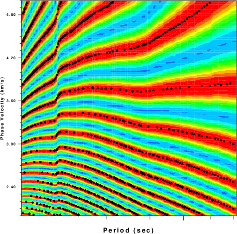 Image for Rayleigh wave |
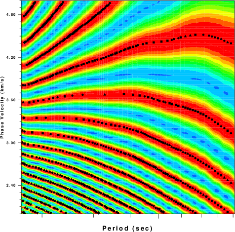 Image for Love wave |
The graphics for the logarithmic period axis lacks labels. This is an easily corrected problem in the PROGRAMS.330/SUBS/grphsubf.f routines that currently only annotate the powers of 10. Currently the only indication is that the 50 second period "tic" is slightly longer. The Rayleigh disperison is vigen from about 15 to 70 seconds which the Love dispersion plot is from about 15 to 90 seconds.
The final thing to note is the "kink" in the Rayleigh dispersion indicates that some other arrival is present, e.g., the phase match filter picked up on noise or some other higher mode.
Fortunately the program sacpom96 creates a shell script that permits an overlay of dispersion onto the file POM96.PLT. For example the outpur for the Love wave exercise created POM96CMP which the shell script DOITT renamed T_POM96CMP:
#!/bin/sh

sdpegn96 -X0  2.00 -Y0  1.00 -XLEN  6.00 -YLEN  6.00 -XMIN   17.0     -XMAX   91.0     -YMIN  2.00 -YMAX  5.00 -PER  -L -C -NOBOX -XLOG -YLIN
If the eigenfunction file slegn96.egn is in the current directory, this will create the plot file SLEGNC.PLT that can be plotted on top of the T_POM96.PLT. We would like to overlay some independent dispersion instead. To do this we modify the shell script to read as sollows:
#!/bin/sh

sdpdsp96 -X0  2.00 -Y0  1.00 -XLEN  6.00 -YLEN  6.00 -XMIN   17.0     -XMAX   91.0     -YMIN  2.00 -YMAX  5.00 -PER  -L -C -NOBOX -XLOG -YLIN -K 0 -S 0.05 -D GDM52.dsp
to create the file SLDSPC.PLT. The dispersion gile GDM52.dsp is from a modified form of Ekstrom's GDM52 distribution. the resultant figures are as follow:
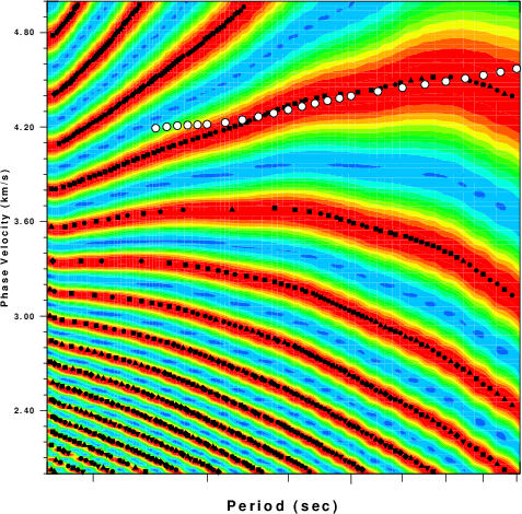 Overlay of Ekstrom's global dispersion onto the output of do_pom96 for the Rayleigh wave fundamental mode. |
 Overlay of Ekstrom's global dispersion onto the output of do_pom96 for the Love wave fundamental mode. |
Note that I used Ekstrom's code to get the dispersion between the two stations, which is only approimate. I should have obtained the dispersion between the epicenter and the two stations, and then estimated the dispersion between the two great circle distances, which is what do_pom96 does.