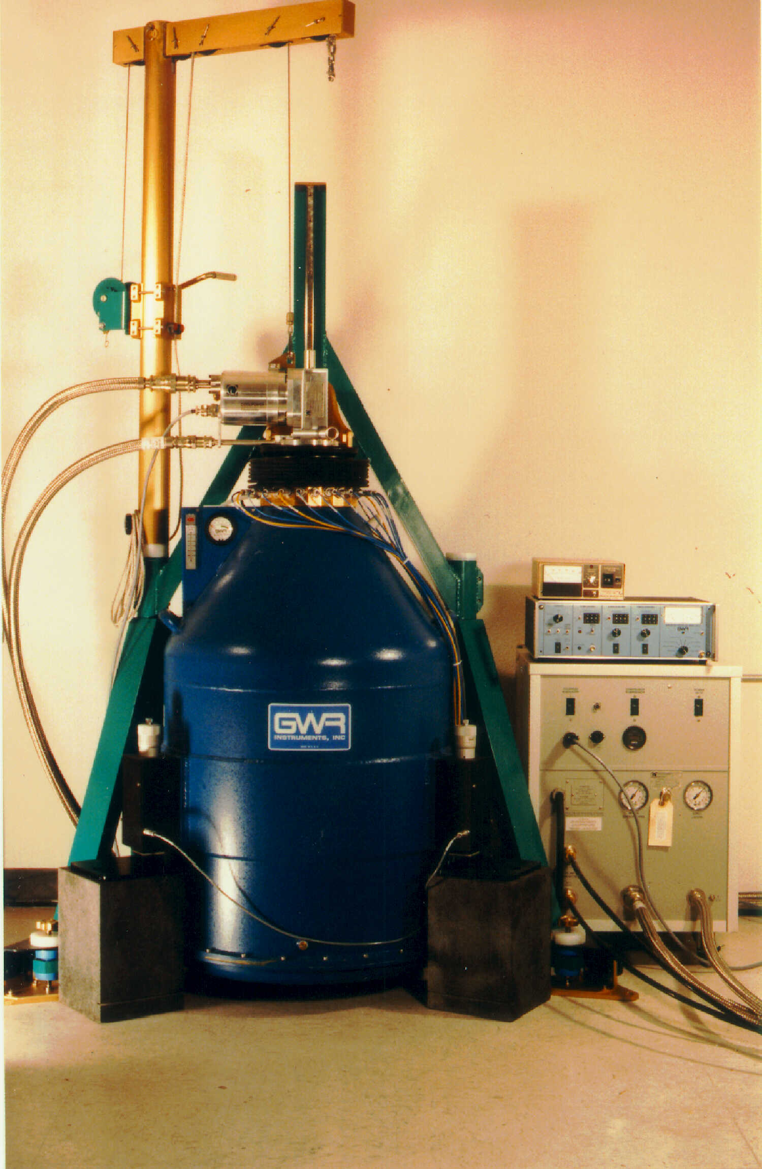
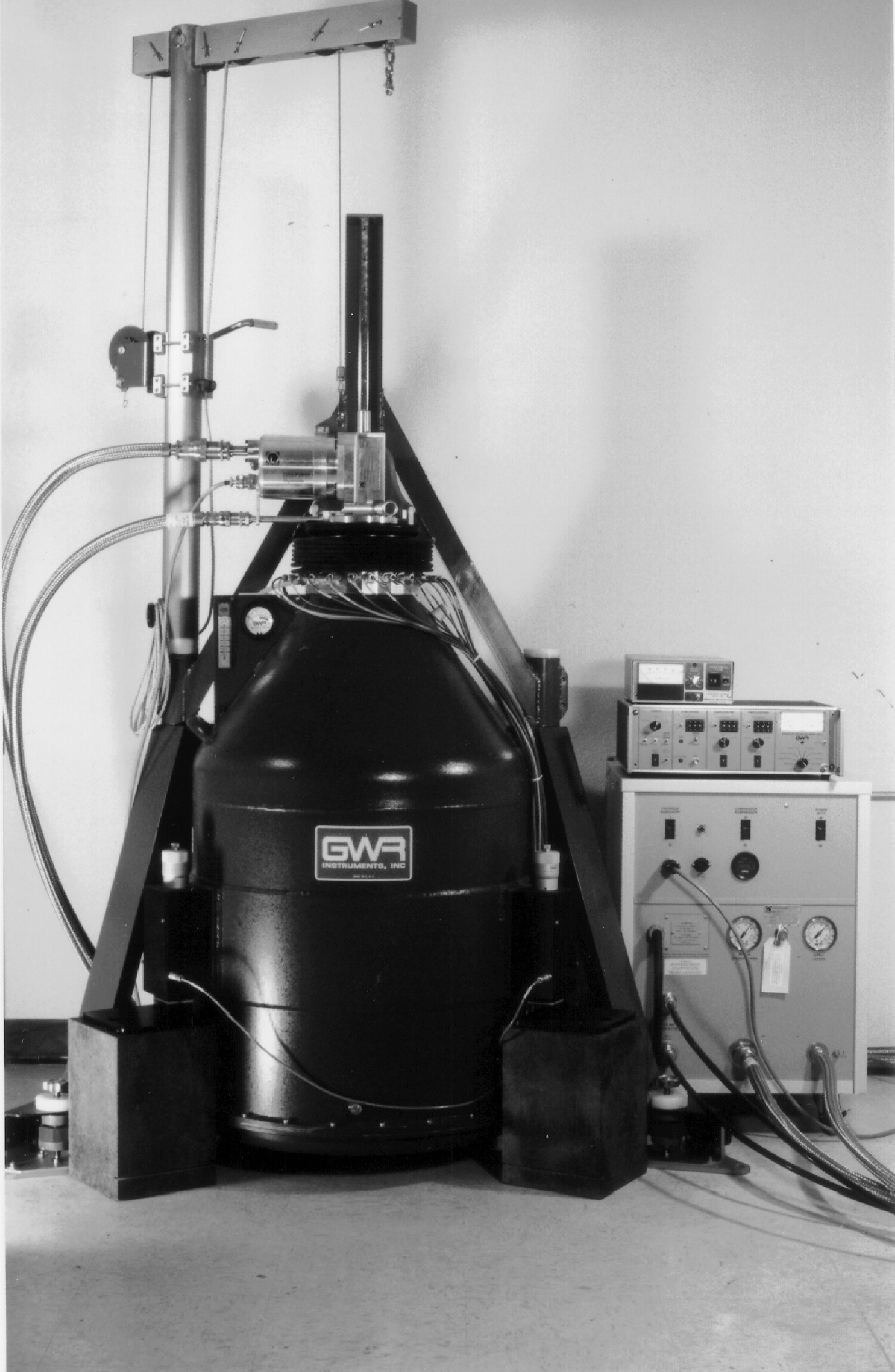
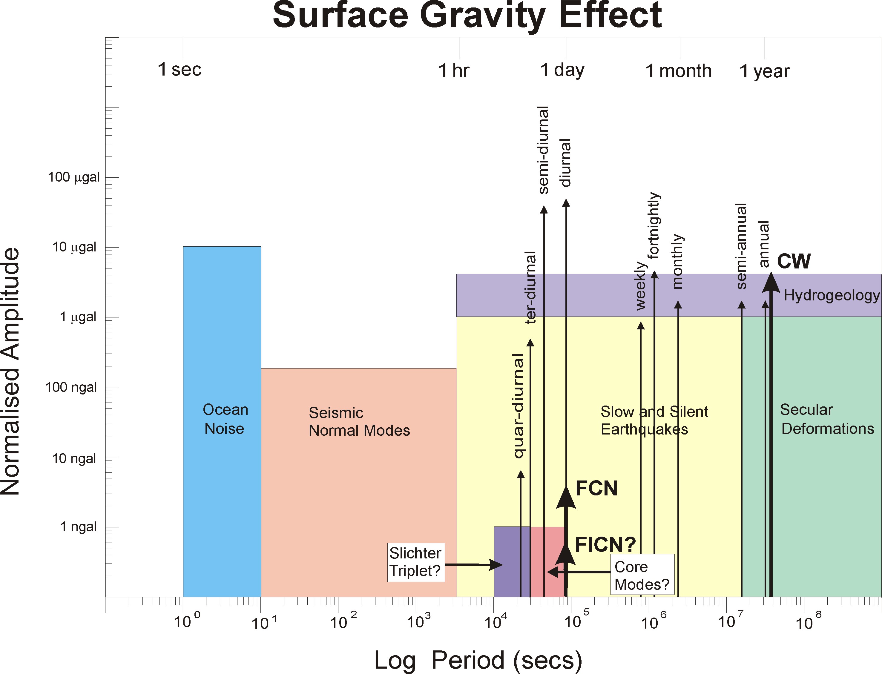
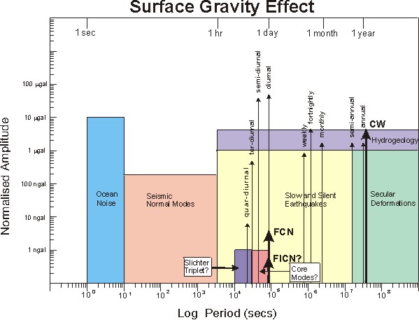
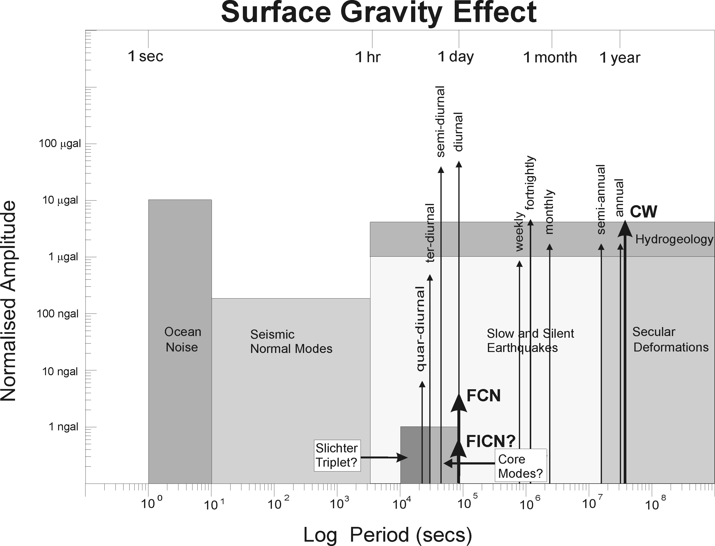
EOS Figures

The following figures are the same as in the article (EOS). We have included some new data replacing the original Figure 4(a).

Figure 1. One of the new generation of Compact Tidal SGs, manufactured by GWR Instruments (San Diego). The sensor uses a Nb superconducting test mass which is levitated in a magnetic field created by superconducting coils. The extremely low noise and low drift are primarily due to the operation of the components at liquid He temperatures regulated to a few micro-Kelvin inside a vacuum can. The model (CT-D) shown is equipped with 2 vertically spaced sensors to measure gravity and gravity gradient. A special refrigeration unit allows the instrument to be run indefinitely with only one filling of liquid He. All aspects of the CT-D can be monitored remotely by modem (high res color | low res color | b&w).

Figure 2. The GGP network showing currently recording stations (high res color | low res color | b&w).

Figure 3. Representation of the gravimetric effect of various signals mentioned in the text at mid-latitudes, using harmonic amplitude normalization. We have omitted the atmospheric pressure effect because the amplitude of the background variability is dependent on the record length. Likewise the ocean tidal loading, also not shown, is highly station dependent. Both of these signals have significant strength at tidal line frequencies (high res color | low res color | b&w).

Figure 4. Examples of long period gravity variations determined by SGs: (a) 500 days from Strasbourg (ST), showing agreement between IERS polar motion, SG and absolute gravimeter data, (b) 200 days from Boulder (BO), showing how rainfall and computed groundwater can account for significant gravity changes, and (c) 900 days from Syowa station, Antarctica (SY), showing that long term gravity changes can be well modeled (high res color | low res color| b&w).

New Figures

Figure 4(a) (above) in the EOS article shows a comparison between two kinds of gravimeter data - superconducting (SG) and absolute (AG) - with IERS polar motion. Unfortunately, due to processing errors, the RMS deviations in the SG data are of the order of 3-4 mgal, of the same order as the error bars for the AG data. In fact the RMS deviations in the SG data are closer to 1 mgal, as demonstrated by the new figures (above).

Figure 5(a) (high res color | low res color | b&w) shows similar AG and SG data to that in the EOS figure, but the SG data is obtained using a more reliable processing. Note that the polar motion is subtracted from both data sets and the time span of the new plot is longer than that in the EOS figure. The residual signal in the SG data is now of the order of 1 mgal, whereas the AG data is the same as the EOS figure (except for 2 new points). Agreement between the 2 data sets is very good and both track real signals at the 3-5 mgal level.

To verify that this comparison is not limited to one site, the second example, Figure 5(b) (high res color | low res color | b&w) shows similar data from Boulder Colorado, of a 2 year comparison between C024 (SG) and AG data from several FG5s. Tides, atmospheric pressure, polar motion and the SG drift have been removed. Again the residual SG noise fluctuates around 1 mgal and common gravity signals of the order of 5 mgal are seen in both data sets. In this case the SG and AG data have had their mean values removed for the time periods; the SG data has not been optimally adjusted to the level of the AG.

Both examples indicate that SG residual gravity fluctuations are at the 1 mgal level and compare well with the slightly noisier AG data with errors of several mgal. More detailed comparisons between the 2 sensors of the latest generation of GWR SGs (shown elsewhere on the GGP Web site) suggest that gravity variations as small as a few tenths of a mgal can be reliably identified as of geophysical rather than instrumental origin.

David Crossley and Jacques Hinderer, April 1999.